![]()
Multiscale Permutation Entropy using feature relevance analysis for vibration-based condition monitoring
Case Western Reserve Experiments
Database link: https://engineering.case.edu/bearingdatacenter
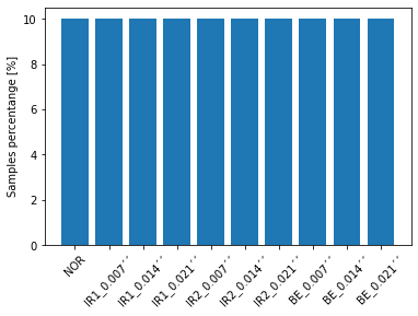
Vibration signals were collected according to the following conditions (classes): i) Normal bearing (Nor), fault in the internal train (IR1), fault in the external train (IR2), and fault in the rolling element-ball (BE). Moreover, the failure states were produced with three levels of severity (0.007′′, 0.014′′, and 0.021′′) and three operating speeds (1730, 1750, 1772, and 1797 [rpm]). Each experiment was repeated three times, and the data was collected at 12 kHz for 5 seconds. Each signal was divided into ten sub-signals.
Accordingly, \(F_s=12k\) [Hz], \(N = 1200\), \(T = 4096\), \(C = 10\).
[8]:
!git clone https://github.com/Jectrianama/GCCE_TEST.git
fatal: destination path 'GCCE_TEST' already exists and is not an empty directory.
[9]:
from sklearn.preprocessing import LabelBinarizer
from sklearn.preprocessing import OneHotEncoder
from scipy.stats import mode
import numpy as np

def ook(t):
  lb = LabelBinarizer()
  y_ook = lb.fit_transform(t)

  if len(np.unique(t))==2:
    y_ook = np.concatenate((1-y_ook.astype(bool), y_ook), axis = 1)

  return y_ook
Loading Data
[10]:
#data downloaded for google drive
FILEID = "1IC11LrPCZIo_Am5eXP2p2tDAlrGTlPjn"
!wget --load-cookies /tmp/cookies.txt "https://docs.google.com/uc?export=download&confirm=$(wget --quiet --save-cookies /tmp/cookies.txt --keep-session-cookies --no-check-certificate 'https://docs.google.com/uc?export=download&id='$FILEID -O- | sed -rn 's/.*confirm=([0-9A-Za-z_]+).*/\1\n/p')&id="$FILEID -O datos.zip && rm -rf /tmp/cookies.txt
!unzip -o datos.zip
!dir
database = 'Western'
--2023-02-11 05:21:53--  https://docs.google.com/uc?export=download&confirm=t&id=1IC11LrPCZIo_Am5eXP2p2tDAlrGTlPjn
Resolving docs.google.com (docs.google.com)... 173.194.69.138, 173.194.69.102, 173.194.69.113, ...
Connecting to docs.google.com (docs.google.com)|173.194.69.138|:443... connected.
HTTP request sent, awaiting response... 303 See Other
Location: https://doc-10-0s-docs.googleusercontent.com/docs/securesc/ha0ro937gcuc7l7deffksulhg5h7mbp1/fopdreo3kn6c73p8pugva79364dc9frm/1676092875000/09173029842254050324/*/1IC11LrPCZIo_Am5eXP2p2tDAlrGTlPjn?e=download&uuid=2aafbfc8-e04f-4109-ac1c-4122df222236 [following]
Warning: wildcards not supported in HTTP.
--2023-02-11 05:21:54--  https://doc-10-0s-docs.googleusercontent.com/docs/securesc/ha0ro937gcuc7l7deffksulhg5h7mbp1/fopdreo3kn6c73p8pugva79364dc9frm/1676092875000/09173029842254050324/*/1IC11LrPCZIo_Am5eXP2p2tDAlrGTlPjn?e=download&uuid=2aafbfc8-e04f-4109-ac1c-4122df222236
Resolving doc-10-0s-docs.googleusercontent.com (doc-10-0s-docs.googleusercontent.com)... 108.177.119.132, 2a00:1450:4013:c00::84
Connecting to doc-10-0s-docs.googleusercontent.com (doc-10-0s-docs.googleusercontent.com)|108.177.119.132|:443... connected.
HTTP request sent, awaiting response... 200 OK
Length: 125624679 (120M) [application/zip]
Saving to: ‘datos.zip’

datos.zip           100%[===================>] 119.80M   208MB/s    in 0.6s

2023-02-11 05:21:55 (208 MB/s) - ‘datos.zip’ saved [125624679/125624679]

Archive:  datos.zip
  inflating: Vibra.mat
  inflating: __MACOSX/._Vibra.mat
  inflating: CaractCE.mat
  inflating: __MACOSX/._CaractCE.mat
CaractCE.mat  datos.zip  GCCE_TEST  __MACOSX  sample_data  Vibra.mat
[11]:
import os
os.chdir('/content/GCCE_TEST/Models')
from  keras_ma_gcce import *
from labels_generation import MA_Clas_Gen
os.chdir('../../')
[12]:
#main libraries and functions
import scipy.io as sio
from sklearn.decomposition import PCA
from sklearn.manifold import TSNE
from sklearn.preprocessing import MinMaxScaler, StandardScaler
import numpy as np
import matplotlib.pyplot as plt
from matplotlib.ticker import FormatStrFormatter
import warnings
#compute centroid index
from sklearn.metrics import pairwise_distances
import matplotlib

warnings.filterwarnings('ignore')


def centroid_(X):
  mean_X = X.mean(axis=0)#computing mean along samples
  D = pairwise_distances(mean_X.reshape(1,-1),X)
  return np.argmin(D)#return centroid index


#loading data
path_ = 'CaractCE.mat'#Case Western Database
dicX = sio.loadmat(path_)
[13]:
dicX.keys()
[13]:
dict_keys(['__header__', '__version__', '__globals__', 'CE', 'E', 'F'])
[14]:
Xt = dicX['F'] #time segments
Fs = 12000 #sampling frequency
Tl = Xt.shape[1]/Fs
print('Xt shape:',Xt.shape)
print('Time length [s]', Tl)
Xt shape: (1200, 4000)
Time length [s] 0.3333333333333333
Multiscale permutation entropy was calculated for each time segment, fixing the delay within [xx,xx] and the embedding time within the range [xx,xxx]. See MPEVA.py for details.
Loading MPE features, time segments, and labels
[15]:
#loading precalculated MPE features
X = dicX['CE']
print('MPE feature matriz shape:',X.shape)
MPE feature matriz shape: (1200, 125)
[16]:
Y = dicX['E']
Ytrue = Y[:,2] #target classes

labels_ = ['NOR','IR1_0.007´´','IR1_0.014´´','IR1_0.021´´',
           'IR2_0.007´´','IR2_0.014´´','IR2_0.021´´',
           'BE_0.007´´','BE_0.014´´','BE_0.021´´'
           ] #classes name

#histogram
unique_elements, counts_elements = np.unique(Ytrue, return_counts=True)
plt.bar(unique_elements,100*counts_elements/X.shape[0])
plt.xticks(unique_elements)
plt.ylabel('Samples percentange [%]')
plt.gca().set_xticklabels(labels_,rotation=45)
plt.show()
[17]:
#rpm labels
nrpm = 30
Yrpm_b = np.r_[0*np.ones(nrpm),np.ones(nrpm),2*np.ones(nrpm),3*np.ones(nrpm)]
Yrpm_b.shape
Yrpm = Yrpm_b
for i in range(len(labels_)-1):
  Yrpm = np.r_[Yrpm,Yrpm_b]
[18]:
Y = np.c_[Y,Yrpm]
[19]:
import joblib

CaseWestern_data = {'Xdata_time' : Xt, 'Fs' : Fs,
                    'Xdata_MPE' : X, 'Y_labels' : Y}

joblib.dump(CaseWestern_data,"CasaWestern_data.pkl")
[19]:
['CasaWestern_data.pkl']
[20]:
Y.shape
[20]:
(1200, 4)
[21]:
Y
[21]:
array([[ 0.,  0.,  1.,  0.],
       [ 0.,  0.,  1.,  0.],
       [ 0.,  0.,  1.,  0.],
       ...,
       [ 1.,  3., 10.,  3.],
       [ 1.,  3., 10.,  3.],
       [ 1.,  3., 10.,  3.]])
Interpretability results
[22]:
Xt.shape
[22]:
(1200, 4000)
[23]:
#scatter plots
scar = StandardScaler()
sca = MinMaxScaler()
red = TSNE(perplexity = 10,n_components=2,random_state=123)
vt = np.arange(0,Tl,1/Fs)
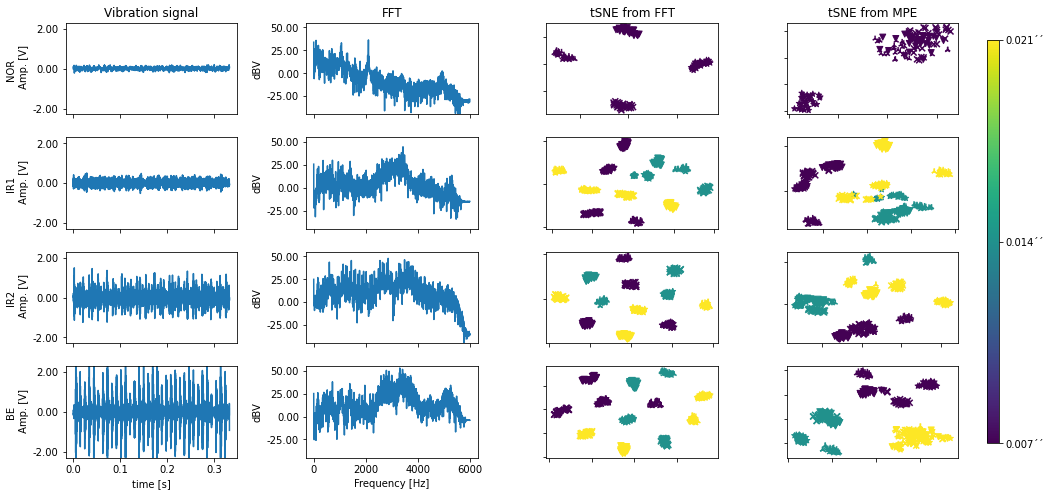
Ytrue_f = Y[:,1] # labels = [Normal, Internal, External, Ball]
labels_f = ['NOR', 'IR1', 'IR2', 'BE']
#scatter along fault lables
fig, axs = plt.subplots(len(labels_f),4,figsize=(16, 8))
j=0
vf = np.fft.rfftfreq(Xt.shape[1],1/Fs) #freq vector
Xw = 20*np.log10(abs(np.fft.rfft(Xt))) # FFT
marker_s = ['2','v','x','*'] # RPM1, RPM2, RPM3, RPM4 as marker changes
for i in np.unique(Ytrue_f):
X_ = Xt[Ytrue_f==i]
Xw_ = Xw[Ytrue_f==i]
XE_ = X[Ytrue_f==i]
Z_ = scar.fit_transform(red.fit_transform(sca.fit_transform(Xw_)))
Z_e = scar.fit_transform(red.fit_transform(sca.fit_transform(XE_)))
#identify centroid RPM1
ind = centroid_(Z_[Yrpm[Ytrue_f==i] == 0])
#time plots
axs[j,0].plot(vt,X_[ind])
axs[j,0].set_ylim([-2.3,2.3])
axs[j,0].yaxis.set_major_formatter(FormatStrFormatter('%.2f'))
axs[j,0].set_ylabel(labels_f[j]+' \n Amp. [V]')
if j!=len(labels_f)-1: axs[j,0].set_xticklabels([])
#frequency plots
axs[j,1].plot(vf,Xw_[ind])
axs[j,1].set_ylim([-45,55])
axs[j,1].yaxis.set_major_formatter(FormatStrFormatter('%.2f'))
axs[j,1].set_ylabel('dBV')
if j!=len(labels_f)-1: axs[j,1].set_xticklabels([])
#scatter plots
cc = Ytrue[Ytrue_f==i]
#FFT-based features scatter plot
for ii in np.unique(Yrpm):
ind_ = Yrpm[Ytrue_f==i] == ii
im = axs[j,2].scatter(Z_[ind_,0],Z_[ind_,1],c=cc[ind_],marker=marker_s[int(ii)])
#axs[j,2].scatter(Z_[ind,0],Z_[ind,1],c='r',marker='v')
axs[j,2].set_xticklabels([])
axs[j,2].set_yticklabels([])
#MPE-based features scatter plot
im = axs[j,3].scatter(Z_e[ind_,0],Z_e[ind_,1],c=cc[ind_],marker=marker_s[int(ii)])
#axs[j,3].scatter(Z_e[ind,0],Z_e[ind,1],c='r',marker='v')
axs[j,3].set_xticklabels([])
axs[j,3].set_yticklabels([])
j+=1
cax = fig.add_axes([0.925, 0.15, 0.01, 0.7])
norm = matplotlib.colors.Normalize(vmin=0,vmax=2)
sm = plt.cm.ScalarMappable(cmap=None, norm=norm)
sm.set_array([])
cbar = plt.colorbar(sm,cax=cax,ticks=[0, 1, 2])
cbar.ax.set_yticklabels(['0.007´´', '0.014´´', '0.021´´'])
axs[-1,0].set_xlabel('time [s]')
axs[-1,1].set_xlabel('Frequency [Hz]')
axs[0,0].set_title('Vibration signal')
axs[0,1].set_title('FFT')
axs[0,2].set_title('tSNE from FFT')
axs[0,3].set_title('tSNE from MPE')
fig.subplots_adjust(wspace=0.4, hspace=0.25)
plt.show()
[24]:
#X.shape
[25]:
Ytrue.min()
#X = Xw
[25]:
1
[26]:
X.shape
[26]:
(1200, 125)
[27]:
Y, iAnn, Lam_r = MA_Clas_Gen(X ,Ytrue, R=5, NrP=1)

[28]:
Y = Y - 1
t = Ytrue- 1
[29]:
import pandas as pd
from sklearn.metrics import classification_report
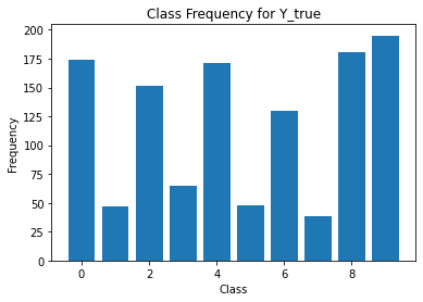
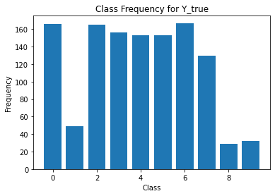
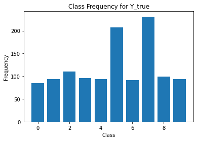
for i in range(Y.shape[1]):
print('annotator',i+1)
print(classification_report(t,Y[:,i]))
unique, counts = np.unique(Y[:,i], return_counts=True)
plt.figure()
plt.bar(unique, counts)
# unique, counts = np.unique(Y_test[5], return_counts=True)
# plt.bar(unique, counts)
plt.title('Class Frequency for Y_true')
plt.xlabel('Class')
plt.ylabel('Frequency')
annotator 1
              precision    recall  f1-score   support

           0       0.82      1.00      0.90       120
           1       0.83      1.00      0.91       120
           2       0.77      0.39      0.52       120
           3       0.84      0.90      0.87       120
           4       0.00      0.00      0.00       120
           5       0.82      1.00      0.90       120
           6       0.88      1.00      0.93       120
           7       0.81      1.00      0.90       120
           8       0.86      0.99      0.92       120
           9       0.87      1.00      0.93       120

    accuracy                           0.83      1200
   macro avg       0.75      0.83      0.78      1200
weighted avg       0.75      0.83      0.78      1200

annotator 2
              precision    recall  f1-score   support

           0       0.69      1.00      0.82       120
           1       0.00      0.00      0.00       120
           2       0.63      0.79      0.70       120
           3       0.17      0.09      0.12       120
           4       0.70      1.00      0.82       120
           5       0.02      0.01      0.01       120
           6       0.64      0.69      0.66       120
           7       0.00      0.00      0.00       120
           8       0.66      0.99      0.79       120
           9       0.62      1.00      0.76       120

    accuracy                           0.56      1200
   macro avg       0.41      0.56      0.47      1200
weighted avg       0.41      0.56      0.47      1200

annotator 3
              precision    recall  f1-score   support

           0       0.72      1.00      0.84       120
           1       0.43      0.17      0.25       120
           2       0.73      1.00      0.84       120
           3       0.75      0.97      0.85       120
           4       0.78      1.00      0.88       120
           5       0.78      1.00      0.88       120
           6       0.72      1.00      0.84       120
           7       0.71      0.77      0.74       120
           8       0.03      0.01      0.01       120
           9       0.00      0.00      0.00       120

    accuracy                           0.69      1200
   macro avg       0.57      0.69      0.61      1200
weighted avg       0.57      0.69      0.61      1200

annotator 4
              precision    recall  f1-score   support

           0       0.72      1.00      0.84       120
           1       0.45      0.33      0.38       120
           2       0.69      0.88      0.77       120
           3       0.66      0.98      0.79       120
           4       0.70      1.00      0.82       120
           5       0.03      0.01      0.01       120
           6       0.72      1.00      0.84       120
           7       0.00      0.00      0.00       120
           8       0.03      0.01      0.01       120
           9       0.69      0.97      0.81       120

    accuracy                           0.62      1200
   macro avg       0.47      0.62      0.53      1200
weighted avg       0.47      0.62      0.53      1200

annotator 5
              precision    recall  f1-score   support

           0       0.00      0.00      0.00       120
           1       0.00      0.00      0.00       120
           2       0.14      0.12      0.13       120
           3       0.00      0.00      0.00       120
           4       0.00      0.00      0.00       120
           5       0.57      0.99      0.73       120
           6       0.00      0.00      0.00       120
           7       0.52      1.00      0.68       120
           8       0.00      0.00      0.00       120
           9       0.00      0.00      0.00       120

    accuracy                           0.21      1200
   macro avg       0.12      0.21      0.15      1200
weighted avg       0.12      0.21      0.15      1200


[30]:
import numpy.matlib
from sklearn.model_selection import ShuffleSplit, StratifiedShuffleSplit
Ns = 1
ss = ShuffleSplit(n_splits=Ns, test_size=0.3,random_state =123)
for train_index, test_index in ss.split(X):
    print(test_index)
    X_train, X_test,Y_train,Y_test = X[train_index,:], X[test_index,:],Y[train_index,:], Y[test_index,:]
    Y_true_train, Y_true_test = t[train_index].reshape(-1,1), t[test_index].reshape(-1,1)
print(X_train.shape, Y_train.shape, Y_true_train.shape)
[ 156  920  971  897   35  599  567  553  891 1010  524  440 1141  579
  138  566 1186  172  961  610  662  186  134  418  427  245  571  226
  348 1071  637  203 1136  210  701  879  314  448 1088  406  375 1011
  972  694  167  654 1069  678  982 1026  591 1195 1105  690  528  800
  987  568  935   42  476  693  758  486   97  299  746  305    5  490
  336  310  600  968  511  565   72  587  702  656   18   13  774  807
  960  895  802 1117 1044  279  664   67  512  921  136 1157  150 1085
   69  923  384 1106  964  456  825  204  318  196  362  887  417   85
 1051  278  209  499 1019  154  779  844  351  739   98  560  462   86
   45  590  304  228  898  332  103  882  688  429  178  319 1043  822
 1182  294  188  943  229 1114   68  177  621  677 1123  507  376 1007
  787  810  141  756 1033  163  120  240  976  252   95  529  352  431
  617  309  437  870  161  902  772  627  681  266  861  206  909  725
  221 1130 1116 1148  801  768  948  580  754  805 1119  373  973  594
  839   84 1055  409 1135 1045  182  624  710  307  249  714  603  586
  184  536  119  444  280 1154 1151  326  260  989  316  856 1100  733
 1178  502 1198  198  145  685  812  674  453   31  811 1015  250  282
  651   43 1048  738   15  777  171  933  543 1066  129  200  367 1013
 1075  875  263 1072   50  723  986 1073  251  306  394  831  611  883
  396  558  643  776  541 1171  244  372  109 1173  303  657    9  842
  683  157  147   65  190  243  289  820    7  112  789  131 1127  164
 1074  794  613  235  684  452  682  906  124  647  876  917  176  916
 1050   90  905   57   40 1101  292  267  965  646 1125  421 1056  130
  110  670   33 1124  966  668  208  114 1077 1143  706  399  212   52
 1115  904 1049   41  300  907  614  764  705  854  261  598  616  663
  491  388  732  727  274  356  869  317 1145  497]
(840, 125) (840, 5) (840, 1)
[31]:
scaler = MinMaxScaler()
scaler.fit(X_train)
X_train = scaler.transform(X_train)
X_test = scaler.transform(X_test)
[32]:
from sklearn.metrics import classification_report, balanced_accuracy_score, roc_auc_score
from sklearn.metrics import normalized_mutual_info_score, mutual_info_score, adjusted_mutual_info_score
l1 =0.01
NUM_RUNS =10
ACC = np.zeros(NUM_RUNS)
AUC = np.zeros(NUM_RUNS)
AUCSK = np.zeros(NUM_RUNS)
MI = np.zeros(NUM_RUNS)
NMI = np.zeros(NUM_RUNS)
AMI = np.zeros(NUM_RUNS)
BACC = np.zeros(NUM_RUNS)
for i in range(NUM_RUNS): #10
print("iteration: " + str(i))
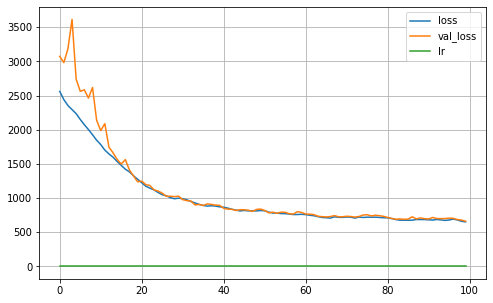
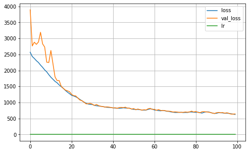
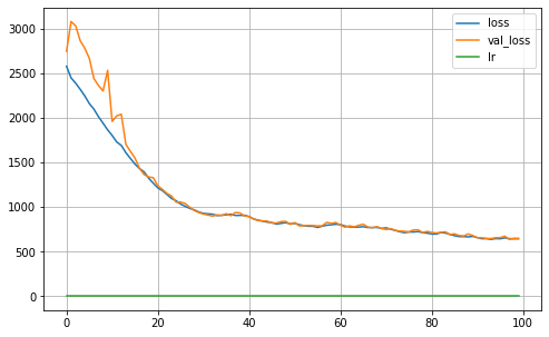
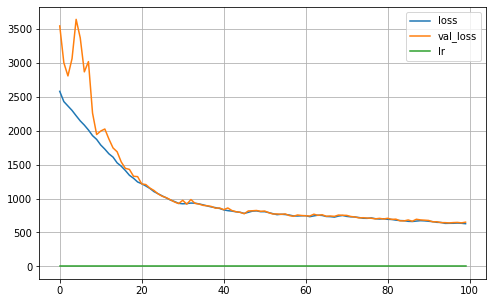
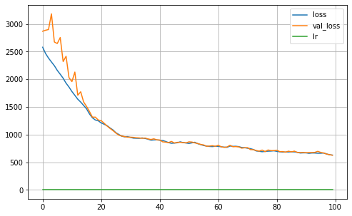
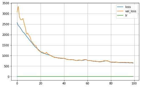
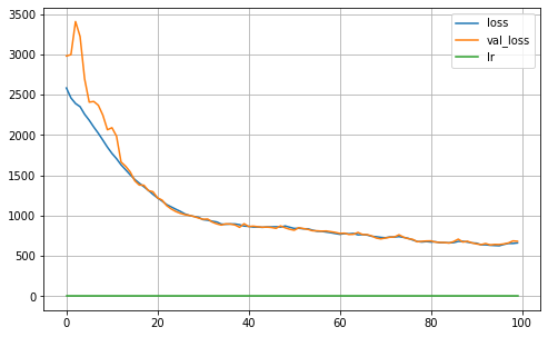
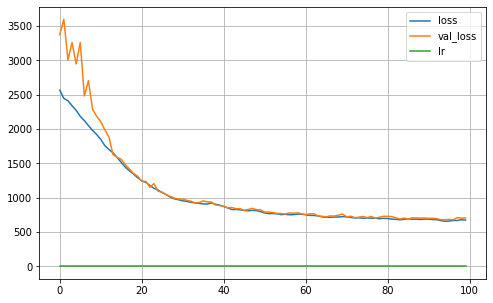
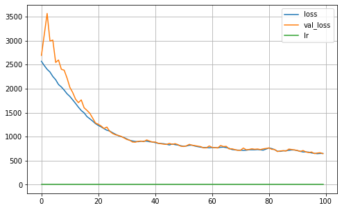
MA = Keras_MA_GCCE(epochs=100,batch_size=64,R=5, K=len(np.unique(Y_true_train)), dropout=0.25, learning_rate=0.001,optimizer='Adam',
l1_param=l1, validation_split=0.30, verbose=0, q=0.01, neurons=4)
MA.fit(X_train, Y_train)
MA.plot_history()
#Accuracy
pred_2 = MA.predict(X_test)
report = classification_report( pred_2[:,Y.shape[1]:].argmax(axis=1),Y_true_test.ravel(),output_dict=True)
ACC[i] = report['accuracy']
print("Validation ACC: %.4f" % (float(ACC[i])))
# balanced. Accurcy
BACC[i] = balanced_accuracy_score(Y_true_test.squeeze(), pred_2[:,Y.shape[1]:].argmax(axis=1).squeeze(), adjusted=True)
print("Validation Balanced_ACC: %.4f" % (float(BACC[i])))
#MI
MI[i] = mutual_info_score(Y_true_test.squeeze(), pred_2[:,Y.shape[1]:].argmax(axis=1).squeeze())
print("Validation MI: %.4f" % (float(MI[i]),))
NMI[i] = normalized_mutual_info_score(Y_true_test.squeeze(), pred_2[:,Y.shape[1]:].argmax(axis=1).squeeze())
print("Validation Normalized MI: %.4f" % (float(NMI[i]),))
AMI[i]= adjusted_mutual_info_score(Y_true_test.squeeze(), pred_2[:,Y.shape[1]:].argmax(axis=1).squeeze())
print("Validation Adjusted MI: %.4f" % (float(AMI[i]),))
#AUC
val_AUC_metric = tf.keras.metrics.AUC( from_logits = True)
# val_logits =MA.predict(X_test) # model(X_test, training=False)
# tf.print(y_batch_val)
val_AUC_metric.update_state(Y_true_test, pred_2[:,Y.shape[1]:].argmax(axis=1).astype('float'))
val_AUC = val_AUC_metric.result()
val_AUC_metric.reset_states()
val_AUC = val_AUC.numpy()
print("Validation aUc: %.4f" % (float(val_AUC),))
AUC[i] = val_AUC
val_AUC1 = roc_auc_score(ook(Y_true_test), pred_2[:,Y_train.shape[1]:])
print("Validation aUc_Sklearn: %.4f" % (float(val_AUC1),))
AUCSK[i] = val_AUC1
iteration: 0
12/12 [==============================] - 0s 21ms/step
Validation ACC: 0.9889
Validation Balanced_ACC: 0.9895
Validation MI: 2.2471
Validation Normalized MI: 0.9795
Validation Adjusted MI: 0.9784
Validation aUc: 1.0000
Validation aUc_Sklearn: 0.9996
iteration: 1
12/12 [==============================] - 1s 40ms/step
Validation ACC: 0.9778
Validation Balanced_ACC: 0.9722
Validation MI: 2.2150
Validation Normalized MI: 0.9674
Validation Adjusted MI: 0.9655
Validation aUc: 1.0000
Validation aUc_Sklearn: 0.9997
iteration: 2

12/12 [==============================] - 0s 24ms/step
Validation ACC: 0.9861
Validation Balanced_ACC: 0.9870
Validation MI: 2.2387
Validation Normalized MI: 0.9757
Validation Adjusted MI: 0.9743
Validation aUc: 1.0000
Validation aUc_Sklearn: 0.9998
iteration: 3
12/12 [==============================] - 0s 24ms/step
Validation ACC: 0.9806
Validation Balanced_ACC: 0.9762
Validation MI: 2.2215
Validation Normalized MI: 0.9698
Validation Adjusted MI: 0.9681
Validation aUc: 1.0000
Validation aUc_Sklearn: 0.9986
iteration: 4
12/12 [==============================] - 0s 23ms/step
Validation ACC: 0.9889
Validation Balanced_ACC: 0.9897
Validation MI: 2.2510
Validation Normalized MI: 0.9812
Validation Adjusted MI: 0.9801
Validation aUc: 1.0000
Validation aUc_Sklearn: 0.9994
iteration: 5
12/12 [==============================] - 1s 39ms/step
Validation ACC: 0.9861
Validation Balanced_ACC: 0.9828
Validation MI: 2.2355
Validation Normalized MI: 0.9757
Validation Adjusted MI: 0.9744
Validation aUc: 1.0000
Validation aUc_Sklearn: 0.9979
iteration: 6
12/12 [==============================] - 0s 25ms/step
Validation ACC: 0.9778
Validation Balanced_ACC: 0.9709
Validation MI: 2.2177
Validation Normalized MI: 0.9691
Validation Adjusted MI: 0.9673
Validation aUc: 1.0000
Validation aUc_Sklearn: 0.9988
iteration: 7
12/12 [==============================] - 0s 23ms/step
Validation ACC: 0.9861
Validation Balanced_ACC: 0.9841
Validation MI: 2.2358
Validation Normalized MI: 0.9756
Validation Adjusted MI: 0.9742
Validation aUc: 0.9985
Validation aUc_Sklearn: 1.0000
iteration: 8
12/12 [==============================] - 0s 24ms/step
Validation ACC: 0.9694
Validation Balanced_ACC: 0.9590
Validation MI: 2.1963
Validation Normalized MI: 0.9615
Validation Adjusted MI: 0.9593
Validation aUc: 1.0000
Validation aUc_Sklearn: 0.9964
iteration: 9
12/12 [==============================] - 0s 23ms/step
Validation ACC: 0.9889
Validation Balanced_ACC: 0.9895
Validation MI: 2.2471
Validation Normalized MI: 0.9795
Validation Adjusted MI: 0.9784
Validation aUc: 1.0000
Validation aUc_Sklearn: 0.9983
[33]:
ACC
[33]:
array([0.98888889, 0.97777778, 0.98611111, 0.98055556, 0.98888889,
       0.98611111, 0.97777778, 0.98611111, 0.96944444, 0.98888889])
[34]:
AUC
[34]:
array([1.        , 1.        , 1.        , 1.        , 1.        ,
       1.        , 1.        , 0.99846154, 1.        , 1.        ])
[35]:
print('Average Accuracy: ', np.round( ACC.mean(),4)*100)
print('Average std: ',np.round(np.std( ACC),4)*100)
Average Accuracy:  98.31
Average std:  0.61
[36]:
print('Average Accuracy: ', np.round( AUC.mean(),4)*100)
print('Average std: ',np.round(np.std( AUC),4)*100)
Average Accuracy:  99.98
Average std:  0.05
[37]:
print('Average Accuracy: ', np.round( ACC.mean(),4)*100)
print('Average std: ',np.round(np.std( ACC),4)*100)
print('==============================================')
print('Average AUC: ', np.round( AUC.mean(),4)*100)
print('Average AUC std: ',np.round(np.std( AUC),4)*100)
print('==============================================')
print('Average AUC Sklearn: ', np.round( AUCSK.mean(),4)*100)
print('Average AUC SK std: ',np.round(np.std( AUCSK),4)*100)
print('==============================================')
print('Average Balanced Accuracy: ', np.round( BACC.mean(),4)*100)
print('Average std: ',np.round(np.std( BACC),4)*100)
print('==============================================')
print('Average MI: ', np.round( MI.mean(),4)*100)
print('Average std: ',np.round(np.std(MI),4)*100)
print('==============================================')
print('Average Normalized MI: ', np.round( NMI.mean(),4)*100)
print('Average std: ',np.round(np.std(NMI),4)*100)
print('==============================================')
print('Average Ajdusted MI: ', np.round( AMI.mean(),4)*100)
print('Average std: ',np.round(np.std(AMI),4)*100)
Average Accuracy:  98.31
Average std:  0.61
==============================================
Average AUC:  99.98
Average AUC std:  0.05
==============================================
Average AUC Sklearn:  99.89
Average AUC SK std:  0.11
==============================================
Average Balanced Accuracy:  98.00999999999999
Average std:  0.97
==============================================
Average MI:  223.06
Average std:  1.66
==============================================
Average Normalized MI:  97.35000000000001
Average std:  0.6
==============================================
Average Ajdusted MI:  97.2
Average std:  0.63
[38]:
import pickle

# create the dictionary with 6 scalar variables
Metrics = {
    'Accuracy': np.round( ACC.mean(),4)*100,
    'Accuracy_std': np.round(np.std( ACC),4)*100,
    'AUC': np.round( AUC.mean(),4)*100,
    'AUC_std': np.round(np.std( AUC),4)*100,
    'Balanced Accuracy': np.round( BACC.mean(),4)*100,
    'Balanced Accuracy_std':  np.round(np.std(BACC),4)*100,
    'MI': np.round( MI.mean(),4)*100,
    'MI_std': np.round(np.std(MI),4)*100,
    'Normalized MI': np.round( NMI.mean(),4)*100,
    'Normalized MI_std': np.round(np.std(NMI),4)*100,
    'Adjusted MI': np.round( AMI.mean(),4)*100,
    'Adjusted MI_std': np.round(np.std(NMI),4)*100,
}

# save the dictionary to a file using pickle
with open('data.pickle', 'wb') as handle:
    pickle.dump(Metrics, handle, protocol=pickle.HIGHEST_PROTOCOL)